Statistical Inference

Statistical inference is the process of drawing conclusions about populations or scientific truths from data.

Population : All Possible Value
Parameter : A characteristic of population

Data : A subset (Sample) from the Population
Statistic : Calculated from data in the sample

# PP — Parameter is to population, SS — sample is to Statistic

Procedures for making inferences —

1. Estimation
2. Hypotheses testing

Estimation : — The objective of Estimation is to determine the value of a population parameter on the basis of a sample statistic.

Type of Estimation: —

1. Point Estimation
2. Interval Estimation

Point Estimator: — A Point Estimator draws inference about a population by estimating the value of an unknown parameter using a single value or a point.

Interval Estimator: — An Interval Estimator draws inferences about a population by estimating the value of an unknown parameter using an interval.

A Point Estimator is any function W(X1, X2,… , Xn) of a sample; that is , any statistic is a point estimator.

An Estimator is a function of the sample , while an Estimate is the realized value of an estimator

An Interval Estimate of a real — valued parameter Ɵ is any pair of functions , L(x1, x2,… ,xn) and U(x1, x2,… ,xn), of a sample that satisfy L(X) < U(X) for all x . If X=x is observed, the inference L(x)<= Ɵ <=u(x) is made. The random interval [L(X),U(X)] is called interval estimator.

Estimation Methods : Method of Moments: — The method of moments is a technique for estimating the parameters of a statistical model.

The basic idea of this method is to equate certain sample characteristics, such as the mean, to the corresponding population expected values.

Let x1, x2 , x3. . . , xn be a random sample from a PMF or PDF f(x). For k = 1, 2, 3, . . . , the kth population moment, or kth moment of the distribution f(x), is E(Xk).

kth sample moment

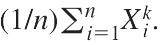
First population moment is E(X) = μ(mean), and the first sample moment is ΣXi/n =x̅

The second population and sample moments are E(X^2) and ΣXi^2/n, respectively. The population moments will be functions of any unknown parameters θ1, θ2, . . . ., θm.

Let X1, X2, . . . , Xn be a random sample from a distribution with pmf or pdf f (x; θ1, . . . , θm), where θ1, . . . , θm are parameters whose values are unknown.

Then the moment estimators θ1, . . . , θm are obtained by equating the first m sample moments to the corresponding first m population moments and solving for θ1, . . . , θm.

for example, if `m = 2, E(X) and E(X^2) will be functions of θ1 and θ2.

Setting E(X) = (1/n) ΣXi (x̅) and E(X^2) = (1/n) Σ Xi^2 gives two equations in θ1 and θ2. The solution then defines the estimators.

Let X1, X2, . . . , Xn represent a random sample of service times of n customers at a certain facility, where the underlying distribution is assumed exponential with parameter λ.

Since there is only one parameter to be estimated, the estimator is obtained by equating E(X) to x̅

Since E(X) = 1/λ for an exponential distribution, this gives 1/λ= or λ = 1/x̅. The moment estimator of λ is then λ=1/x̅

Estimation Methods : Maximum Likelihood Estimation

Maximum likelihood estimation is a method that determines values for the parameters of a model.

A sample of ten new bike helmets manufactured by a certain company is obtained. Upon testing, it is found that the first, third, and tenth helmets are flawed, whereas the others are not.

Let p = P(flawed helmet), i.e., p is the proportion of all such helmets that are flawed.

Define (Bernoulli) random variables X1, X2, . . . , X10

Then for the obtained sample, X1 = X3 = X10 = 1 and the other seven Xi’s are all zero.

The probability mass function of any particular Xi is P^Xi*((1-P)^1-Xi), which becomes p if xi = 1 and 1 — p when xi = 0.

Now lets assume that the conditions of various helmets are independent of each other. This implies that the Xi’s are independent, so their joint probability mass function is the product of the individual PMF’s.

Thus the joint PMF evaluated at the observed Xi’s is

f (x1, . . . , x10; p) = p(1 — p)p . . . p = p^3(1 — p)^7

Suppose that p = 0.25.

Then the probability of observing the sample that we actually obtained is (.25**3)*(.75**7): = 0.0020856857299804688.

If instead p = .50, then this probability is (.50)3(.50)7 = .000977.

For what value of p is the obtained sample most likely to have occurred? That is, for what value of p is the joint PMF (EQ 1) as large as it can be? What value of p maximizes EQ1?

Graph of the likelihood (joint PMF)
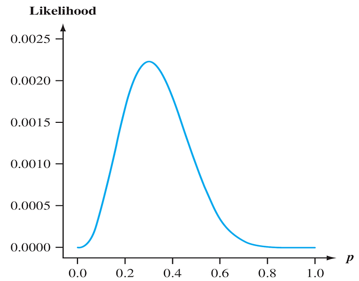
EQ 1 from Example

Figure shows a graph of the likelihood EQ 1 as a function of p. It appears that the graph reaches its peak above p = 0.3, equal to the proportion of flawed helmets in the sample.

We can verify our visual impression by using calculus to find the value of p that maximizes EQ 1.

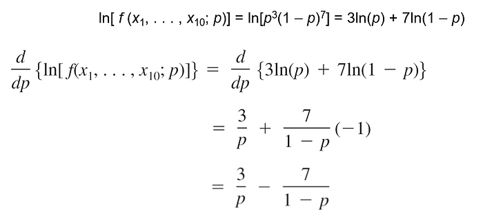
Equating this derivative to 0 and solving for p gives 3(1 — p) = 7p,
from which 3 = 10p and so p = 3/10 = .30

The likelihood function tells us how likely the observed sample is as a function of the possible parameter values.

Maximizing the likelihood gives the parameter values for which the observed sample is most likely to have been generated — that is, the parameter values that “agree most closely” with the observed data.

Thank you for reading. Links to other blogs: —

Bayesian Generalized Linear Model (Bayesian GLM) — 2
Central Limit Theorem — Statistics
General Linear Model — 2
General and Generalized Linear Models
Uniform Distribution
Normal Distribution
Binomial Distribution
10 alternatives for Cloud based Jupyter notebook!!