Probability Distributions 2— Normal Distribution

Probability distribution and Uniform Distribution is already covered in below mentioned Link.

Probability distribution and Uniform Distribution

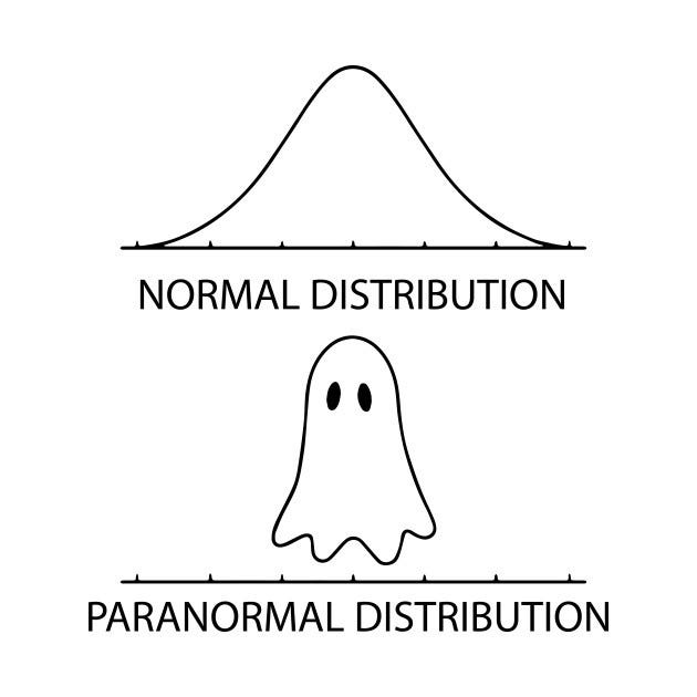
The normal or Gaussian distribution is a continuous probability distribution characterized by a symmetric bell-shaped curve. A normal distribution is defined by its center (mean) and spread (standard deviation.). The bulk of the observations generated from a normal distribution lie near the mean, which lies at the exact center of the distribution: as a rule of thumb, we can think about “The Empirical Rule (Three Sigma Rule)” about 68% of the data lies within 1 standard deviation of the mean, 95% lies within 2 standard deviations and 99.7% lies within 3 standard deviations.

link for three sigma rule blog : — https://medium.com/@yogeshrawat90/the-empirical-rule-three-sigma-rule-7153fe0595db by Yogesh Rawat

The normal distribution is perhaps the most important distribution in all of statistics. It turns out that many real world phenomena, like IQ test scores and human heights, roughly follow a normal distribution, so it is often used to model random variables. Many common statistical tests assume distributions are normal.

The scipy nickname for the normal distribution is norm.

Properties of Normal Distribution

• Mean = median = mode
• Symmetric in nature
• Total area under the curve = 1
• As we move away from the mean, the PDF value decreases
• As the variance increases the distribution spread also increases and the curve becomes more wider
• 68–95–99.7 Empirical rule
• 68.2% of the data lies within one standard deviation away from the mean
• 95% of the data lies within two standard deviation away from the mean
• 99.7% of the data lies within three standard deviation away from the mean

If we know in advance that a variable follows normal distribution then we can easily tell many properties of the variable without looking at the actual data.

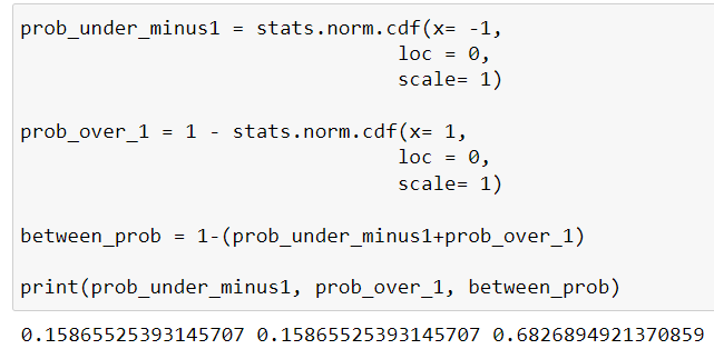
prob_under_minus1 = stats.norm.cdf(x= -1,  
                                loc = 0,               
                                scale= 1)     

prob_over_1 = 1 - stats.norm.cdf(x= 1,  
                                loc = 0,               
                                scale= 1) 

between_prob = 1-(prob_under_minus1+prob_over_1)

print(prob_under_minus1, prob_over_1, between_prob)

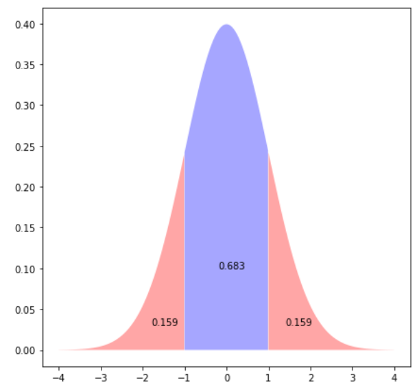
The output shows that roughly 16% of the data generated by a normal distribution with mean 0 and standard deviation 1 is below -1, 16% is above 1 and 68% lies between -1 and 1, which agrees with the 68, 95, 99.7 rule. Let’s plot the normal distribution and inspect areas we calculated:

# Plot normal distribution areas*

plt.rcParams["figure.figsize"] = (9,9)
                                  
plt.fill_between(x=np.arange(-4,-1,0.01), 
                 y1= stats.norm.pdf(np.arange(-4,-1,0.01)) ,
                 facecolor='red',
                 alpha=0.35)

plt.fill_between(x=np.arange(1,4,0.01), 
                 y1= stats.norm.pdf(np.arange(1,4,0.01)) ,
                 facecolor='red',
                 alpha=0.35)

plt.fill_between(x=np.arange(-1,1,0.01), 
                 y1= stats.norm.pdf(np.arange(-1,1,0.01)) ,
                 facecolor='blue',
                 alpha=0.35)

plt.text(x=-1.8, y=0.03, s= round(prob_under_minus1,3))
plt.text(x=-0.2, y=0.1, s= round(between_prob,3))
plt.text(x=1.4, y=0.03, s= round(prob_over_1,3));

The plot above shows the bell shape of the normal distribution, the area below and above one standard deviation and the area within 1 standard deviation of the mean. Finding quantiles of the normal distribution is a common task when performing statistical tests. You can check normal distribution quantiles with stats.norm.ppf():

Normality test

Normality test are used to determine whether the data is normally distribution or not OR whether the sample data comes from normally distributed population or not.
There are various kind of graphical and numeric tests to determine this.

• Graphical tests : — Histogram/density plot and Q-Q plot
• Numeric tests: — Shapiro-Wilk test andKolmogorov-Smironv test

Link to some other blogs: —
Uniform Distribution
Central Limit Theorem
Decision Tree and its types
10 alternatives for Cloud based Jupyter notebook!!
Number System in Python