Central Limit Theorem — Statistics

3 min readFeb 21, 2022

Central Limit Theorem (CLT) is very fundamental and a key concept in probability theory. In this blog we will cover Central Limit Theorem.

CLT theory states that given a sufficiently large sample size from a population with a finite level of variance, the mean of all samples from the same population will be approximately equal to the mean of the population.

if you sample randomly from a population repeatedly, and for each sample you compute an average value over that sample, that the distribution of the averages is Normal Distribution.

Averages of all numbers will be independent of each other and tend to have bell-shaped distributions.

•After fetching different samples, which are enough in numbers, we can then calculate the mean of each sample and then plot the various distributions.

Also, if we take the average of the sample mean, then the result will be equal to the actual population mean & the standard deviation equals σ/√n (Standard Error).

Standard Error (SE) of a statistic is the standard deviation of its sampling distribution or an estimate of that standard deviation.

In Simple words, a sample mean deviates from the actual mean of a population.

Population sample criteria for Central Limit Theorem

Samples should be: -
1.Representative of the population.
2.Big enough to draw conclusions from, which in statistics is a sample size greater or equal to 30.
3.Include less than 10% of the population.
4.The distribution of the original dataset does not matter. However, the distribution of the sample means would be Normal Distribution

Above picture, shows 3 different population distributions which are not normal. Sampling distribution of means gets a little closer to normal distribution when we take n =5 and almost normal distribution when n=30.

Example:

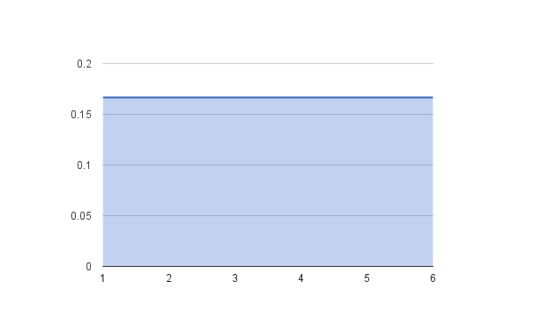
Imagine rolling a 1–6 die lots of times. We expect to get (over a long time) an equal proportion of each roll.

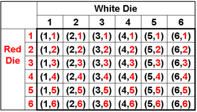
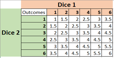
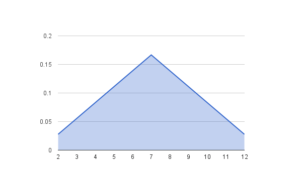
Now lets take two fair dice (One is white and other is red). You only have a 1 in 36 (around 0.03) chance of a 2 or a 12 because there’s only 1 way to make a 2 — you need a 1 on both dice. But a seven is much more common — you have a 1 in 6 (around 0.16) chance of a 7