Probability Distributions 1 — Uniform Distribution
Many statistical tools and techniques used in data analysis are based on probability. Probability measures how likely it is for an event to occur on a scale from 0 (the event never occurs) to 1 (the event always occurs). When working with data, variables in the columns of the data set can be thought of as random variables: variables that vary due to chance. A probability distribution describes how a random variable is distributed; it tells us which values a random variable is most likely to take on and which values are less likely.

In statistics, there are a range of precisely defined probability distributions that have different shapes and can be used to model different types of random events. In this lesson we’ll discuss some common probability distributions and how to work with them in Python.
The Uniform Distribution

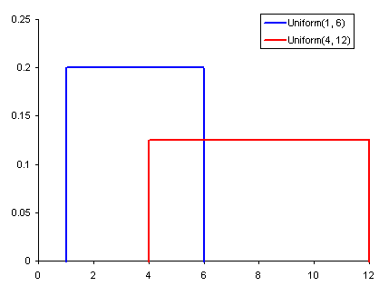
The uniform distribution is a probability distribution where each value within a certain range is equally likely to occur and values outside of the range never occur. If we make a density plot of a uniform distribution, it appears flat because no value is any more likely (and hence has any more density) than another.
Properties
A discrete uniform distribution is a symmetric distribution with following properties.
- It has fixed number of outcomes.
- All the outcomes are equally likely to occur.
If a random variable X follows discrete uniform distribution and it has k discrete values say x1, x2, x3,…..xk, then PMF of X is given as

Many useful functions for working with probability distributions in Python are contained in the scipy.stats library. Let’s load in some libraries, generate some uniform data and plot a density curve:
%matplotlib inline

import numpy as np
import pandas as pd
import matplotlib.pyplot as plt
import scipy.stats as statsuniform_data = stats.uniform.rvs(size=100000,  # Generate 100000 numbers
                                 loc = 0,      # From 0
                                 scale=10)     # To 10pd.DataFrame(uniform_data).plot(kind="density",  # Plot the distribution
                               figsize=(9,9),
                               xlim=(-1,11));

In the code above, we generated 100,000 data points from a uniform distribution spanning the range 0 to 10. In the density plot, we see that the density of our uniform data is essentially level meaning any given value has the same probability of occurring. The area under a probability density curve is always equal to 1.
In this blog we have covered uniform distribution only. We will cover more distributions in upcoming blogs.
Link to some other blogs: —
Central Limit Theorem
Decision Tree and its types
10 alternatives for Cloud based Jupyter notebook!!
Number System in Python
