General Linear Model — 3 — Residual Analysis
A residual is a measure of how far away a point is vertically from the regression line. In simple words, difference between actual and predicted value.
Residual is a diagnostic measure used when assessing the quality of a model. They are also known as errors.

We can check the assumptions of regression by examining the residuals
Examine for linearity assumption (Linearity)
Evaluate independence assumption (Independence of errors)
Evaluate normal distribution assumption (Normality of errors)
Examine for constant variance for all levels of X (homoscedasticity/ Equal variance)
Linearity: The relationship between x and y must be linear. Check this assumption by examining a scatterplot of x and y.
Independence of errors: There should not a relationship between the residuals and the predicted values. We can check this assumption by examining a scatterplot of “residuals versus fits”. The correlation should be approximately 0.
Normality of errors: The residuals must be approximately normally distributed. We can check this assumption by examining a normal probability plot.
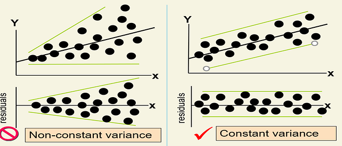
Equal variances: The variance of the residuals should be consistent across all predicted values. We can check this assumption by examining the scatterplot of “residuals versus fits”.
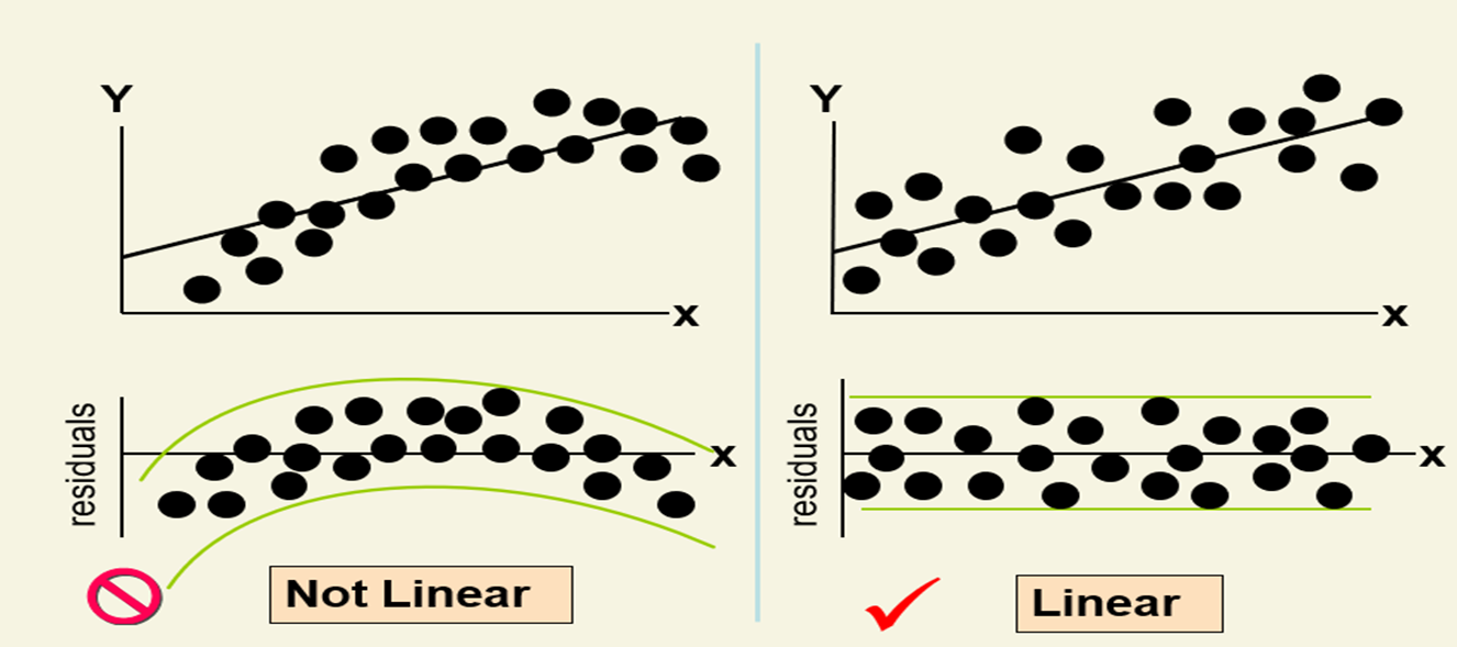
Residual Analysis for Linearity
A residual plot is a graph that shows the residuals on the vertical axis and the independent variable on the horizontal axis. If the points in a residual plot are randomly dispersed around the horizontal axis, a linear regression model is appropriate for the data; otherwise, a nonlinear model is more appropriate.
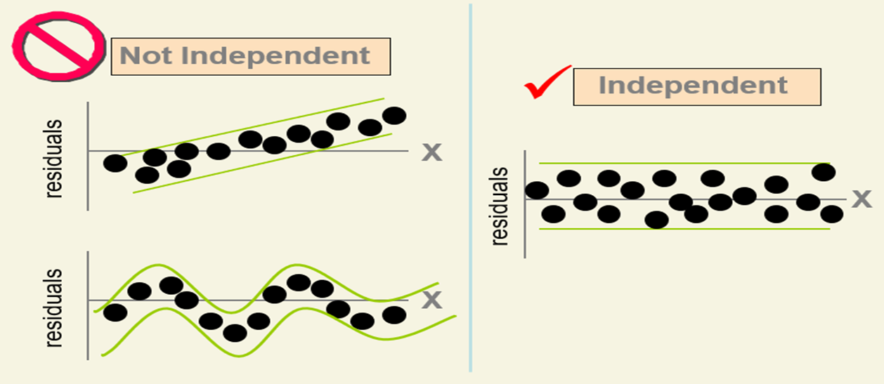
Residual Analysis for Independence
we can plot the residuals vs. the sequential number of the data point. If we notice a pattern, we say that there is an autocorrelation effect among the residuals and the independence assumption is not valid.
Residual Analysis for Independence — Another Method — Durbin Watson (D-W) Statistics
It’s the sum of the squares of the differences between consecutive errors divided by the sum of the squares of all errors.
Another way to look at the Durbin-Watson Statistic is: D = 2(1-ρ)
where ρ = the correlation between consecutive errors.
There are 3 important values for D:
D=0: This means that ρ=1, indicating a positive correlation.
D=2: In this case, ρ=0, indicating no correlation.
D=4: ρ=-1, indicating a negative correlation
Residual Analysis for Equal Variance
- White test statistics
- Residual vs fitted value plot
Checking for Normality
- Examine the Stem-and-Leaf Display of the Residuals.
- Examine the Boxplot of the Residuals
- Examine the Histogram of the Residuals
- Construct a Normal Probability Plot of the Residuals
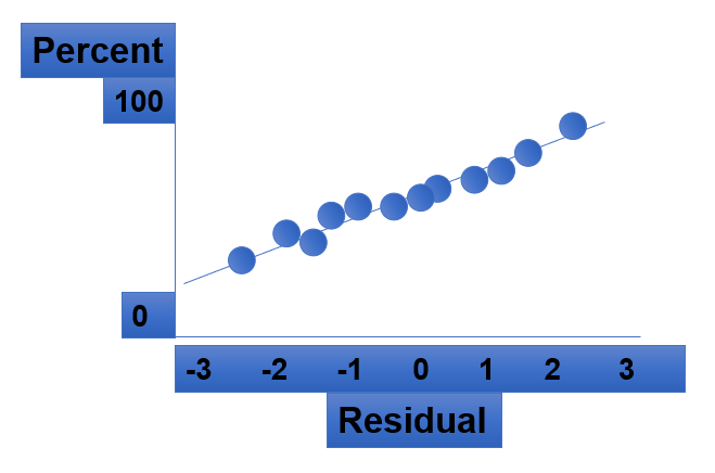
Residual Analysis for Normality
When using a normal probability plot, normal errors will approximately display in a straight line.
Thank you for reading. Links to other blogs: —
General Linear Model — 2
General and Generalized Linear Models
The Poisson Distribution
Uniform Distribution
Normal Distribution
Binomial Distribution
10 alternatives for Cloud based Jupyter notebook!!